
How to Select Distributions in Hydrology — and Where to Find Them
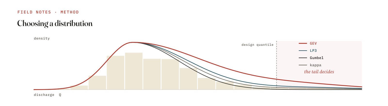
Almost every design number in hydrology is a quantile of a fitted distribution. The 100-year flood, the 7Q10 low flow, the depth–duration–frequency value you size a culvert against — each is a distribution evaluated at a probability. Which means the quietest, most consequential decision in a frequency analysis is the one people spend the least time on: which distribution? Pick the wrong tail and you mis-size the spillway. Here is how I think about it, and where to find the tools that do the fitting.
Start from the variable, not the software
The right family follows from what you are analysing:
- Annual maxima (floods, rainfall depths): the extreme-value families — GEV, Gumbel (EV1, a special case), and Log-Pearson III. LP3 is the United States Bulletin 17C standard for flood frequency; GEV is the more flexible default elsewhere.
- Peaks over threshold: the Generalised Pareto distribution. If you have sub-annual events, POT/GPD uses more of your data than annual maxima and is often the better choice.
- Low flows (e.g. 7-day minima): Weibull or log-normal fits to the annual minima series; remember you are now modelling a lower tail.
- Interarrival times and durations: exponential and gamma families.
- When nothing fits cleanly: the four-parameter kappa distribution is wonderfully flexible and nests several of the above — I use kappa/GEV pulses in my own stochastic streamflow generator precisely because they capture heavy-tailed behaviour the simpler families miss.
Fit with L-moments, not conventional moments
Conventional moments (variance, skew) are dominated by the largest one or two observations — exactly the unstable part of a short hydrological record. L-moments (Hosking and Wallis) are linear combinations of order statistics: far more robust, much better behaved in small samples, and they give you a diagnostic the textbooks underuse — the L-moment ratio diagram. Plot your sample L-skewness against L-kurtosis and see which family’s theoretical curve it falls near. That single picture does more for distribution selection than most formal tests.
Judge the fit where it matters: the tail
Do not select a distribution on a single goodness-of-fit statistic. A Kolmogorov–Smirnov test is dominated by the centre of the data, and the centre is not what you are designing for. Instead:
- Probability plots on the appropriate extreme-value axes — look at how the fit tracks the upper (or lower) tail, where the data is sparse and the design value lives.
- The L-moment ratio diagram for family selection.
- AIC/BIC to compare nested fits, used as a tie-breaker, not an oracle.
- A tail-sensitivity check: refit with the largest event removed and see how much your 100-year estimate moves. If it lurches, say so in the report.
The honest truth is that in the tail — beyond the record — the choice of family dominates the answer more than the parameter estimates do. That uncertainty is real and belongs in your deliverable.
When the record is short, go regional
If at-site data is thin, pool it. Regional frequency analysis (the index-flood method, with Hosking–Wallis homogeneity and discordancy measures) borrows strength across hydrologically similar catchments, fits a common regional growth curve, and scales it by an at-site index. For short records this is almost always better than torturing twelve years of data into a five-parameter fit.
Where to find them
You do not need to code the fits yourself.
- R:
lmomandlmomRFA(L-moments and regional FA),extRemesandevd(extreme-value models),fitdistrplus(general fitting and diagnostics),nsRFA(regional, non-stationary). - Python:
scipy.stats(the workhorse),lmoments3(L-moment estimators),pyextremes(block-maxima and POT with clean diagnostics),scikit-extremes. - Standards-based tools: USGS PeakFQ (Bulletin 17C / LP3) and HEC-SSP for statutory flood-frequency work.
Pick the family from the variable, fit it with L-moments, judge it on the tail, go regional when the record is short — and always report the family, the fitting method, and how much the tail moves when you poke it. The distribution is a modelling decision. Treat it like one.